Final Report

Project Proposal | Midterm Checkpoint | Final Report

Introduction

Kalshi is a regulated prediction market platform where people can buy and sell shares based on whether or not certain events will occur. Users are able to participate in trades on a wide range of topics such as election results, weather conditions, and current events. The price of a contract reflects a collective estimate on how likely something will actually happen.

Prediction markets aggregate information from many participants into continuously updated prices. The prices on these markets can often serve as useful probability estimates for future events and frequently perform well compared with other forecasting methods [1].

However, these markets are not always perfectly calibrated. For example, prediction-market prices can exhibit a favorite–longshot bias, where high-probability outcomes may be underpriced and low-probability outcomes may be overpriced, especially when there is more time remaining before the event resolves. This suggests that raw market prices can still contain systematic distortions [2].

Recently, Kalshi has emerged as a modern regulated prediction market platform and has been studied as a new source of real-time forecasting data. The Federal Reserve found that Kalshi provides high-frequency, continuously updated expectations data that can be valuable for forecasting, especially in macroeconomic settings [3].

This suggests that while Kalshi markets contain useful predictive information, there may still be room for machine learning to improve prediction or calibration by learning patterns from historical market behavior.

Dataset Description + Links

Our dataset contains historical Kalshi market snapshots. Each row is the state of a binary prediction market at a given time (bid/ask prices, volume, and time features), along with the market’s final resolution label.

• Kalshi Finances/Economics 18 Month History

Problem Definition

Although prediction markets are useful indicators, they are not perfectly calibrated or efficient forecasters. The core problem this project aims to solve is the following question:

Can we use early market activity and historical trends to predict a market’s final outcome with greater accuracy than the raw probability implied by current prices?

Kalshi’s real-time expectations already provide valuable insights. With the use of machine learning, we aim to uncover additional patterns from price movements, volume, timing, and other characteristics to forecast better odds. This matters in identifying when market prices are reliable or when they are noisy/inefficient.

Methods

We implemented and compared four different supervised learning approaches to predict target_yes, a binary label indicating whether the market ultimately would resolve to YES. We started with logistic regression and a histogram-based gradient boosting model, then implemented ExtraTrees and weighted ensemble algorithms to improve robustness and probability quality.

Data Processing

The dataset is made up of historical Kalshi market snapshots, where each row is the state of a binary prediction at a given time. The raw data was cleaned and standardized for all models, which included parsing timestamps, normalizing column formatting, imputing missing values, and encoding categorical features.

The target variable is a binary indicator:

target_yes = 1 if the market resolved to YES, and 0 otherwise.

The primary feature groups are:

• Price features: yes_bid, yes_ask, no_bid, no_ask, and last_price, which represent current market-implied probabilities
• Spread and liquidity features: yes_spread, no_spread, liquidity, open_interest, volume_liquidity_ratio
• Volume features: volume, volume_24h, which represent market activity
• Temporal features: minutes_to_expiration, minutes_to_close, which represent how far the market is from resolving
• Lagged features: previous_yes_bid, previous_yes_ask, previous_price, which represent previous price values

We evaluated four supervised models:

• Logistic Regression (which we used as our baseline)
• Histogram-based Gradient Boosting (GBM)
• ExtraTrees
• Weighted ensemble (of calibrated probabilities, dominated by ExtraTrees in this run)

Train / Validation / Test Split

The dataset was partitioned chronologically based on market close time:

• Training set (~70%): the earliest observations were used to fit models
• Validation set (~15%): the intermediate period was used for calibration and model selection
• Test set (~15%): the most recent observations were used for final evaluation of models

A time-based split was used instead of a traditional random split to simulate real-world deployment, where a model would be trained on past data and applied to future markets.

Probability Calibration

• Method: Isotonic Regression
• The model was first trained on the training set
• Then, predictions were generated on the validation set
• The regression model was then fit to map the raw predicted probabilities to calibrated probabilities

This was done to ensure that the predicted probabilities actually reflected the true outcome frequencies. We made sure to do this because our trading policy uses probability differences directly.

Trading Strategy

Our goal was not simply to have as high as a classification accuracy as possible, but rather identify positive expected value trading opportunities.

For each observation:

• The model produced a predicted probability of a YES outcome
• This was then compared to the market probability (which was derived from bid/ask prices)
• An edge was computed based on the difference between the predicted and market probability

A trade was executed if:

edge > threshold

We performed an edge threshold sweep over a range of values to determine an effective trading policy. For each threshold, we computed:

• Total PnL
• Mean PnL per trade
• Trade rate
• Win rate

Results and Discussion

Classification Performance

Model	Split	ROC AUC	Log Loss	Brier
Logistic	Validation	0.746	0.555	0.193
Logistic	Test	0.600	0.820	0.272
GBM	Validation	0.646	0.620	0.221
GBM	Test	0.632	0.611	0.219
ExtraTrees	Validation	0.663	0.583	0.207
ExtraTrees	Test	0.693	0.639	0.215
Weighted ensemble	Validation	0.687	0.583	0.207
Weighted ensemble	Test	0.699	0.623	0.214

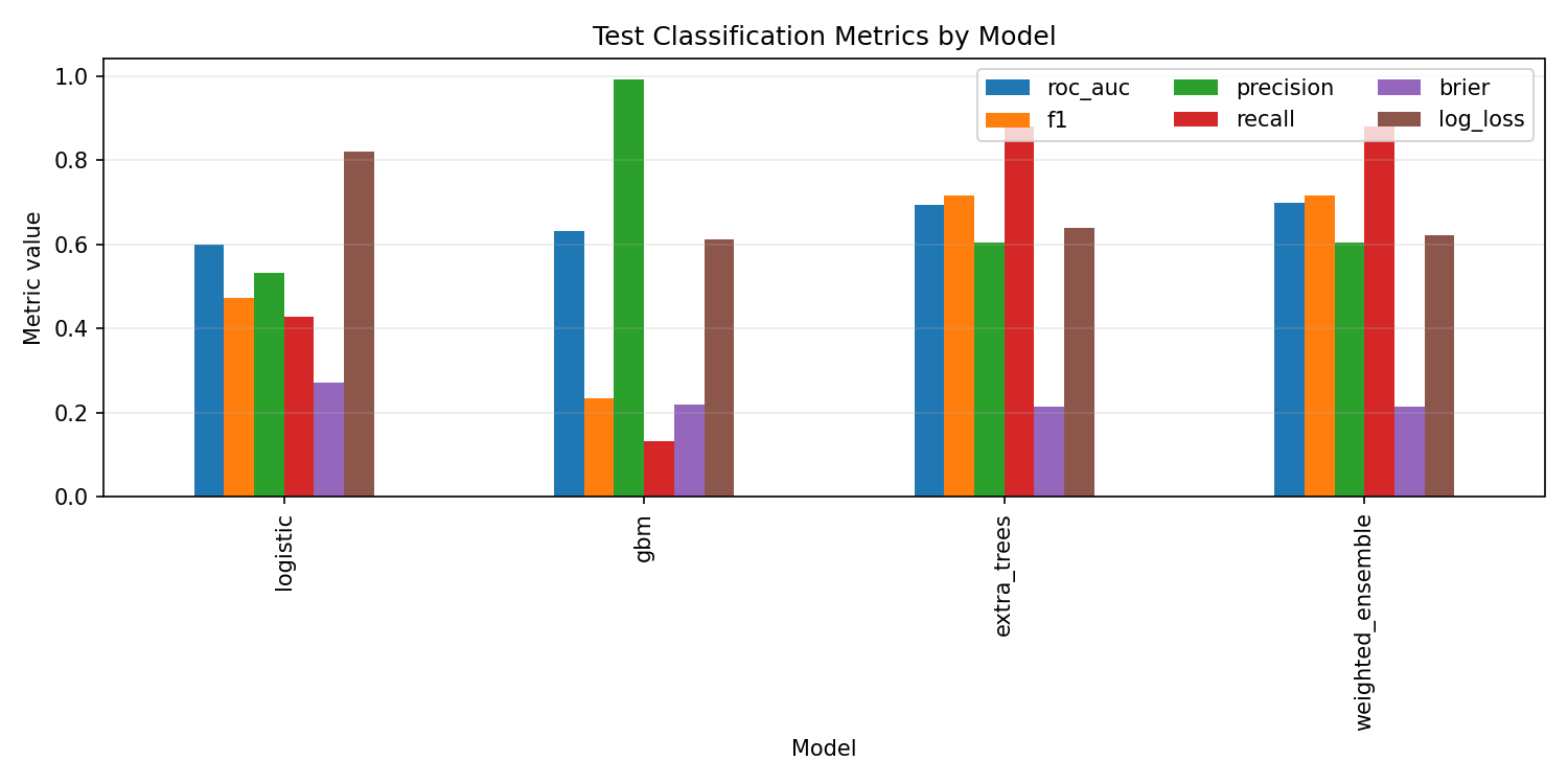Figure 1: Classification metrics on the test split.

These classification results show the same temporal generalization pattern that we noticed earlier on, but now more clearly after we added ExtraTrees and an ensemble. Logistic regression achieved substantially stronger performance on the validation set, but this advantage did not carry over to the test set, where logistic regression had a serious drop in log loss and Brier score, indicating poor out-of-sample probability quality.

Meanwhile, the GBM was comparatively stable between validation and test for log loss/Brier, but the overall AUC was lower than ExtraTrees and the ensemble.

For our more recent models, ExtraTrees performed best amongst the base models on test (highest ROC AUC and improved probability metrics when compared to GBM and logistic). The weighted ensemble was a slight improvement over ExtraTrees on test log loss/Brier and ROC AUC, although the improvement wasn’t groundbreaking because the ensemble was dominated by ExtraTrees in this run.

Trading Performance

Model	Split	Threshold	Total PnL	Mean PnL/Trade	Trade Rate	Win Rate
Logistic	Validation	0.02	25784.87	0.484	0.270	0.488
Logistic	Test	0.02	38278.99	0.487	0.398	0.488
GBM	Validation	0.10	25727.50	0.476	0.274	0.479
GBM	Test	0.10	38339.32	0.519	0.374	0.519
ExtraTrees	Validation	0.02	25841.31	0.494	0.265	0.497
ExtraTrees	Test	0.02	38354.26	0.517	0.376	0.517
Weighted ensemble	Validation	0.02	25843.23	0.493	0.265	0.496
Weighted ensemble	Test	0.02	38357.25	0.517	0.376	0.517

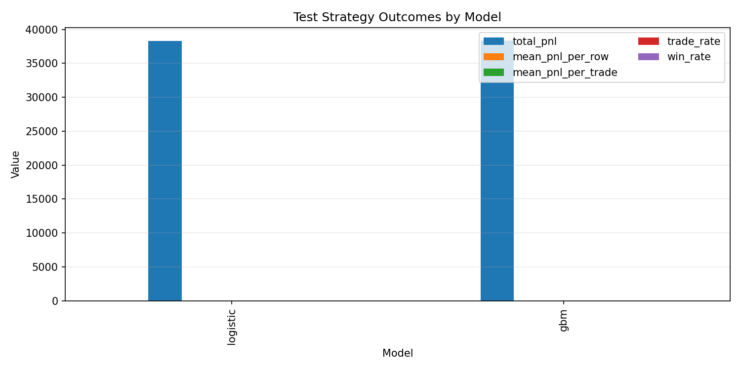Figure 2: Testing Strategy Outcome Differences Between Logistic Regression and GBM

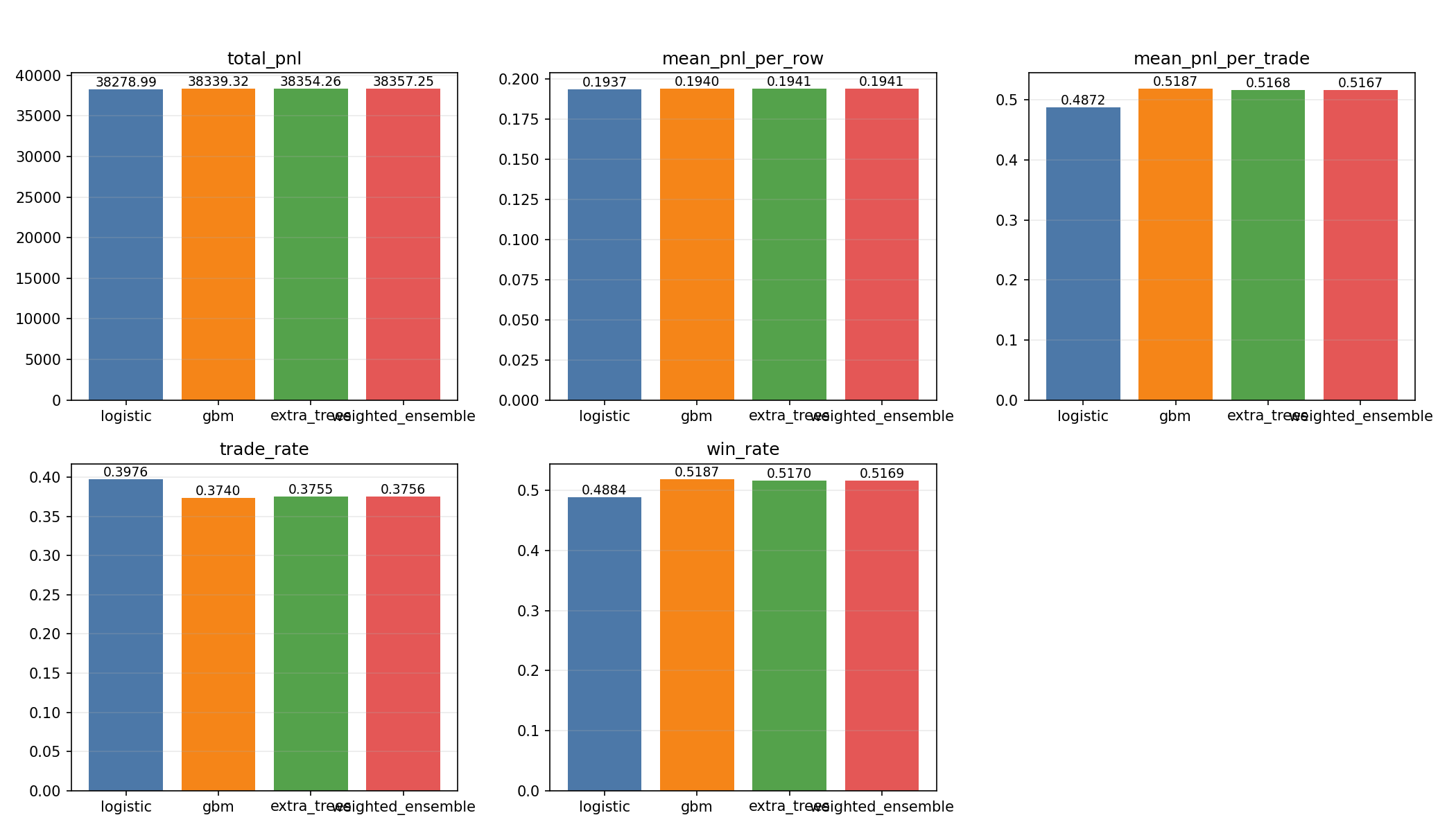Figure 3: PNL, Trade Rate, and Win Rate Differences Across Logistic Regression, GBM, ExtraTrees, and Weighted Ensemble

Despite differences in classification performance, all four models had strong positive expected value under our simplified EV policy. However, their trading behavior were fairly different:

• Logistic regression executed a higher fraction of trades and achieved a lower mean PnL per trade. This indicated a more aggressive strategy relying on volume.
• GBM executed fewer trades but achieved a higher mean PnL per trade and a higher win rate. This suggested that it identified higher-quality opportunities/trades at higher thresholds.
• ExtraTrees and the weighted ensemble achieved the best overall mix of probability quality and trading results, with strong total PnL and improved win rates compared to our baseline model (logistic regression).

Threshold Sensitivity

We performed a threshold sweep on validation to see how sensitive each strategy was to the edge threshold.

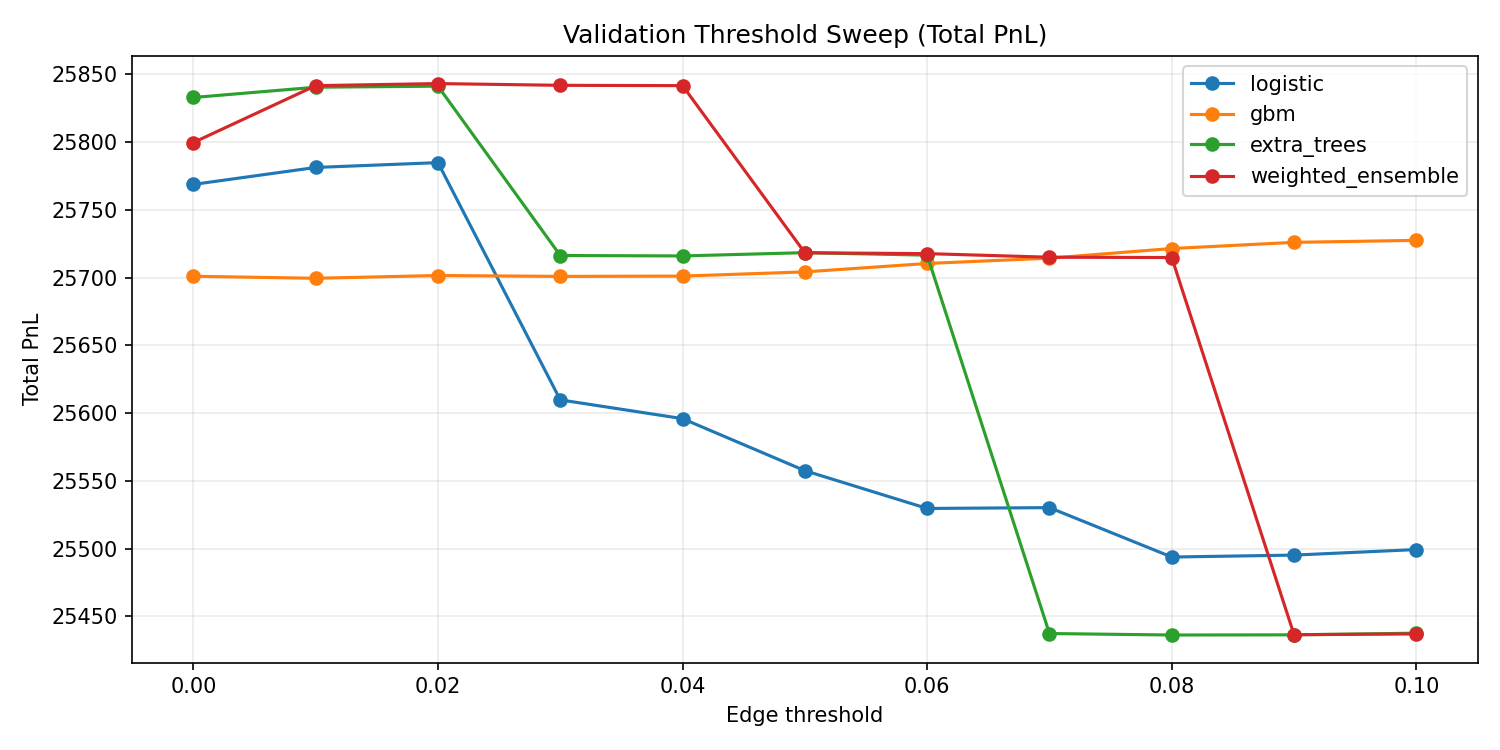
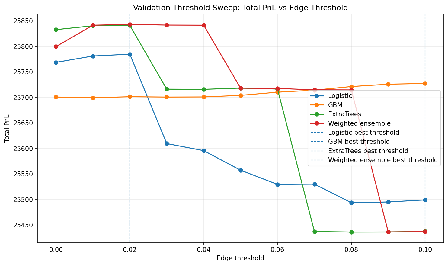Figure 4 and 5: Validation Threshold Sweep Differences Across Logistic Regression, GBM, ExtraTrees, and Weighted Ensemble Models

Interpretation:

• Logistic regression peaked at a relatively low threshold and then exhibited a decrease in performance as the threshold rose, consistent with its test-time miscalibration and unstable probability ranking when dealing with temporal shifts.
• GBM improved steadily as the threshold increased (best around 0.10), suggesting its larger predicted edges corresponded to higher-quality/better trades.
• ExtraTrees and the weighted ensemble were comparatively flat near lower thresholds (best around 0.02 in this run), indicating they found many small edges which remained profitable without requiring additional filtering.

Calibration Analysis

Calibration curves showed whether predicted probabilities matched the observed frequencies.

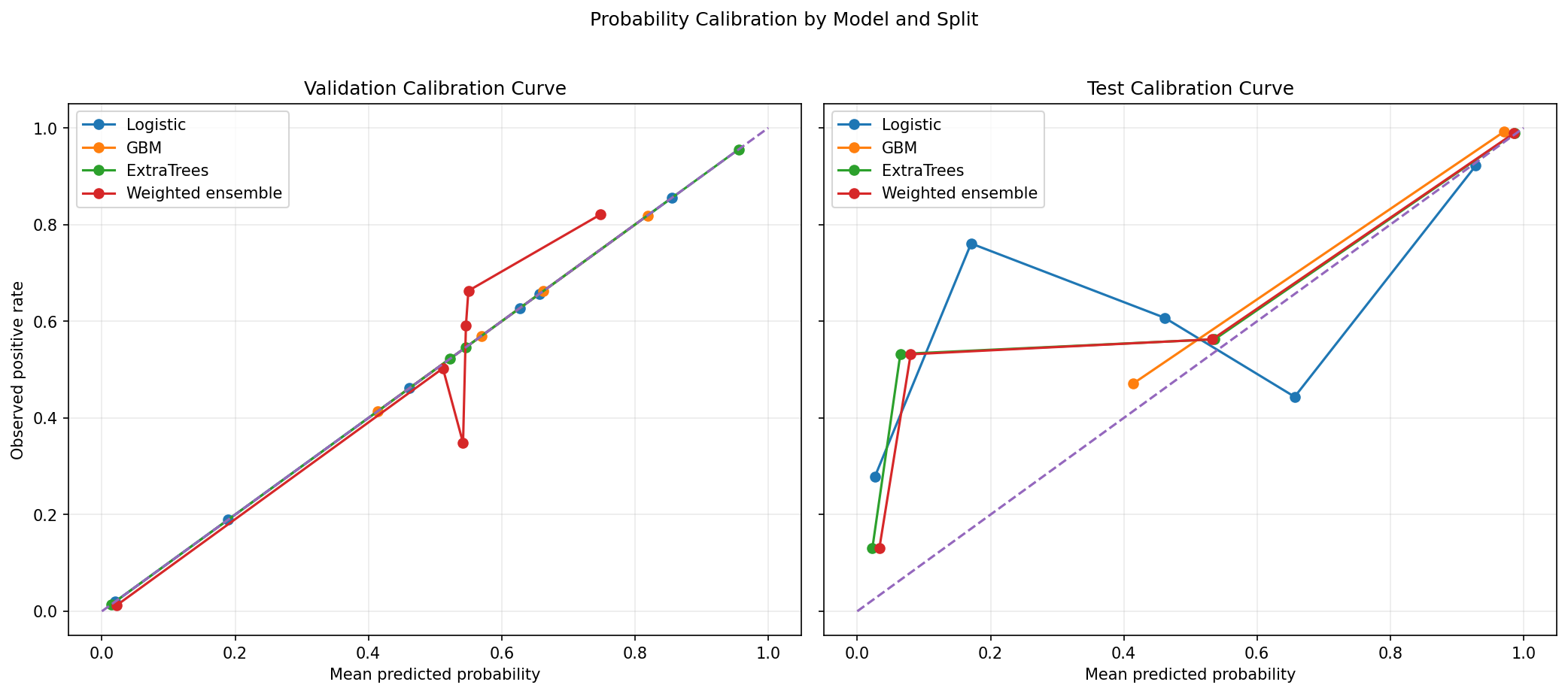Figure 6: Validation and Test Calibration Curve Differences Amongst Logistic Regression, GBM, ExtraTrees, and Weighted Ensemble Models

• Logistic regression was reasonably calibrated during the validation split but deteriorated when it came to the test split. This lines up with its poor test Brier/log loss.
• ExtraTrees and the ensemble were able to maintain closer alignment during the test split, which was important because our strategy depended directly on probability estimates.

Model Interpretability (feature importance)

We used permutation importance on the GBM as a proxy for feature influence.

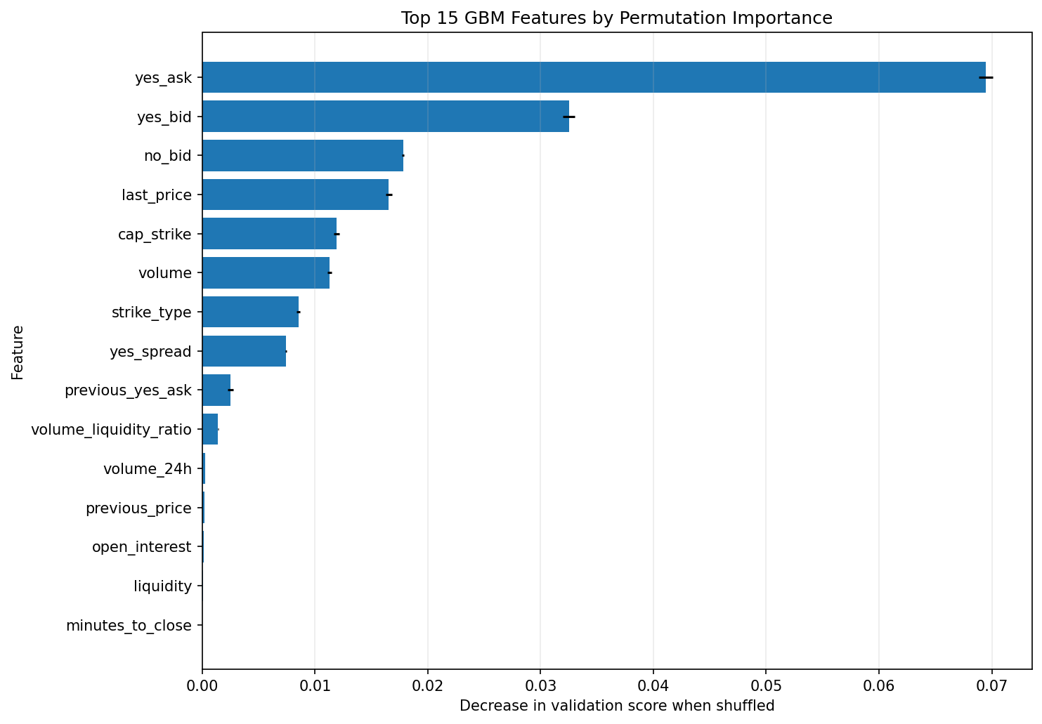Figure 7: Most Important Features for Classification

• The strongest signals came from current market price features (yes_ask, yes_bid, last_price) and liquidity/volume-related context.
• This suggests our models may be actually refining the market rather than predicting independently, which aligns with the idea that prediction markets are informative but imperfectly calibrated.

Limitations + Next Steps

Because our models relied heavily on market price features (i.e. bid/ask), there is some concern that they are simply refining existing market probabilities rather than learning or identifying signals in the data.

Going forward, we think incorporating some exogenous signals (i.e. event timing, category priors, macro/news context) and adding more realistic execution assumptions (fees/slippage) may help address these concerns and improve performance. Additionally, given the way our ensemble was set up, we think there is room for improvement by allowing the model to adjust its weights based on learning from the data (stacking) rather than using a fixed weight vector.

Gantt Chart

Was too large to use screenshot. Can be found here.

Contribution Table

Name	Proposal Contributions
Benjamin Zhao	Report writing/formatting for Github pages + organizing results and figures
Eshaan Patel	Data preprocessing, GBM experiments and evaluation
Liam Weng	Data preprocessing + Logistic regression implementation and evaluation
William Wu	Extratrees + weighted ensemble implementation, figure generation and discussion
Ethan Hu	Threshold sweep analysis, figure generation and discussin

References

1. J. Wolfers and E. Zitzewitz, “Prediction Markets,” Journal of Economic Perspectives, vol. 18, no. 2, pp. 107–126, 2004.

2. L. Page and R. T. Clemen, “Do Prediction Markets Produce Well-Calibrated Probability Forecasts?” The Economic Journal, vol. 123, no. 568, pp. 491–513, 2013.

3. A. M. Diercks, J. D. Katz, and J. H. Wright, “Kalshi and the Rise of Macro Markets,” Finance and Economics Discussion Series, no. 2026-010, Board of Governors of the Federal Reserve System, 2026.